6. Validation
Let’s go through an end-to-end process for training and validating a classification model. After understanding this process, you may modify it for your own purposes. In general, the steps are as follows.
Data: you need to acquire your data relevant to the problem and goal you are trying to achieve; here we generate synthetic data.
Missingness: typically, there is missing data and we need to figure a way to resolve this issue; here, we randomly force data to be missing at random.
Splitting: when we train a model, we desire for the model to be able to
generalizeinto the future againstunseendata; here, we split the data into training and validation sets, where the modeling pipeline will only see the training data and will be tested for performance against the unseen validation set.Training: the training pipeline is dependent on the nature and properties of your data; here, our pipeline is one-hot encoding, imputation, scaling and finally, training a model.
Validation: after we train a model, we evaluate it against unseen data; here, the unseen data is the holdout validation set.
6.1. Generate data
Below, we simulate data D.
\(X_1 \sim \mathcal{N}(0, 1)\)
\(X_2 \sim \mathcal{N}(0, 1)\)
\(X_3\) is
redwhen \(X_1 < 0\) and \(X_2 < 0\)greenwhen \(X_1 > 0\) and \(X_2 > 0\)blueotherwise
\(Y_0 = 1 + 2X_1 + 3X_2 + \sigma\)
\(Y_1 = \frac{1}{1 + \exp(-Y_0)}\)
\(y \sim \mathcal{Binom}(Y_1)\)
[1]:
suppressMessages({
    library('dplyr')
    library('purrr')
})

set.seed(37)

getColor <- function(a, b) {
    if (a < 0 && b < 0) {
        return('red')
    } else if (a > 0 && b > 0) {
        return('green')
    } else {
        return('blue')
    }
}

getData <- function(N=1000) {
    x1 <- rnorm(N, mean=0, sd=1)
    x2 <- rnorm(N, mean=0, sd=1)
    x3 <- map2(x1, x2, getColor) %>% flatten_chr()
    y <- 1 + 2.0 * x1 + 3.0 * x2 + rnorm(N, mean=0, sd=1)
    y <- 1.0 / (1.0 + exp(-y))
    y <- rbinom(n=N, size=1, prob=y)

    df <- data.frame(x1=x1, x2=x2, x3=x3, y=y)
    df <- df %>%
            mutate(y=ifelse(y == 0, 'neg', 'pos')) %>%
            mutate_at('y', as.factor)

    return(df)
}

D <- getData()
[2]:
print(sapply(D, is.factor))
   x1    x2    x3     y
FALSE FALSE  TRUE  TRUE
[3]:
print(head(D))
          x1         x2    x3   y
1  0.1247540  0.4817417 green pos
2  0.3820746  0.8176848 green pos
3  0.5792428 -0.3254274  blue pos
4 -0.2937481 -0.2674061   red pos
5 -0.8283492  1.7163252  blue pos
6 -0.3327136  1.2376945  blue pos
[4]:
print(summary(D))
       x1                x2               x3        y
 Min.   :-2.8613   Min.   :-3.28763   blue :502   neg:394
 1st Qu.:-0.6961   1st Qu.:-0.59550   green:257   pos:606
 Median :-0.0339   Median : 0.06348   red  :241
 Mean   :-0.0184   Mean   : 0.03492
 3rd Qu.: 0.6836   3rd Qu.: 0.69935
 Max.   : 3.8147   Max.   : 3.17901
[5]:
print(dim(D))
[1] 1000 4
6.2. Generate missing data
Here, we make 10% of the data missing in D and store the results in D.M.
[6]:
suppressMessages({
    library('missForest')
})

D.M <- prodNA(D[c('x1', 'x2', 'x3')], noNA=0.1)
D.M$y <- D$y
[7]:
print(summary(D.M))
       x1                 x2               x3        y
 Min.   :-2.86131   Min.   :-3.28763   blue :457   neg:394
 1st Qu.:-0.70096   1st Qu.:-0.61616   green:225   pos:606
 Median :-0.02752   Median : 0.06288   red  :213
 Mean   :-0.03416   Mean   : 0.03213   NA's :105
 3rd Qu.: 0.65422   3rd Qu.: 0.69815
 Max.   : 3.81473   Max.   : 3.17901
 NA's   :102        NA's   :93
[8]:
print(dim(D))
[1] 1000 4
6.3. Split data
Now we split D.M into 80% training D.T and 20% testing D.V.
[9]:
suppressMessages({
    library('caret')
})

trIndices <- createDataPartition(D$y, times=1, p=0.8, list=FALSE)

D.T <- D.M[trIndices, ]
D.V <- D.M[-trIndices, ]
[10]:
print(head(D.T))
          x1         x2    x3   y
1  0.1247540  0.4817417 green pos
2  0.3820746  0.8176848 green pos
3  0.5792428 -0.3254274  blue pos
5         NA  1.7163252  blue pos
7 -0.1921595 -1.1223299   red neg
8  1.3629827  1.5202646  <NA> pos
[11]:
print(head(D.V))
           x1         x2    x3   y
4  -0.2937481 -0.2674061   red pos
6  -0.3327136  1.2376945  blue pos
26 -0.4590474  1.5723978  blue pos
29 -2.1039691  1.0775911  blue pos
33  0.6553955         NA  blue neg
36  0.1297151  0.2434078 green pos
[12]:
print(dim(D.T))
[1] 801 4
[13]:
print(dim(D.V))
[1] 199 4
6.4. Profile data
6.4.1. Statistical profiles
Now, let’s quickly look at the data profiles.
6.4.1.1. Training profile
[14]:
library('skimr')

skimmed <- skim(D.T[,1:2])
s <- skimmed[, c(2:6, 12)]
print(s)
# A tibble: 2 x 6
  skim_variable n_missing complete_rate numeric.mean numeric.sd numeric.hist
  <chr>             <int>         <dbl>        <dbl>      <dbl> <chr>
1 x1                   87         0.891      -0.0156      0.994 ▁▅▇▃▁
2 x2                   73         0.909       0.0337      1.04  ▁▃▇▅▁
[15]:
skimmed <- skim(D.T[,3:4])
s <- skimmed[, c(2:7)]
print(s)
# A tibble: 2 x 6
  skim_variable n_missing complete_rate factor.ordered factor.n_unique
  <chr>             <int>         <dbl> <lgl>                    <int>
1 x3                   81         0.899 FALSE                        3
2 y                     0         1     FALSE                        2
# … with 1 more variable: factor.top_counts <chr>
6.4.1.2. Validation profile
[16]:
skimmed <- skim(D.V[,1:2])
s <- skimmed[, c(2:6, 12)]
print(s)
# A tibble: 2 x 6
  skim_variable n_missing complete_rate numeric.mean numeric.sd numeric.hist
  <chr>             <int>         <dbl>        <dbl>      <dbl> <chr>
1 x1                   15         0.925      -0.106       1.05  ▂▇▇▂▁
2 x2                   20         0.899       0.0257      0.977 ▁▂▇▅▁
[17]:
skimmed <- skim(D.V[,3:4])
s <- skimmed[, c(2:7)]
print(s)
# A tibble: 2 x 6
  skim_variable n_missing complete_rate factor.ordered factor.n_unique
  <chr>             <int>         <dbl> <lgl>                    <int>
1 x3                   24         0.879 FALSE                        3
2 y                     0         1     FALSE                        2
# … with 1 more variable: factor.top_counts <chr>
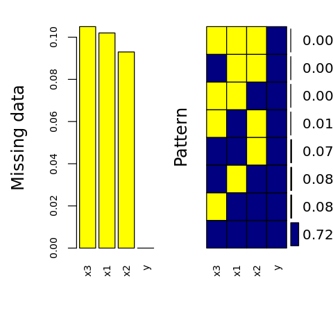
6.4.2. Missingness profiles
Below, we visually inspect the data missingness.
[18]:
suppressMessages({
    library('VIM')
})

options(repr.plot.width=4, repr.plot.height=4)

p <- aggr(
    D.M,
    col=c('navyblue','yellow'),
    numbers=TRUE,
    sortVars=TRUE,
    labels=names(D.M),
    cex.axis=.7,
    gap=3,
    ylab=c('Missing data', 'Pattern')
)
 Variables sorted by number of missings:
 Variable Count
       x3 0.105
       x1 0.102
       x2 0.093
        y 0.000
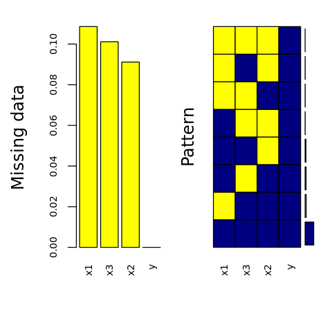
[19]:
p <- aggr(
    D.T,
    col=c('navyblue','yellow'),
    numbers=TRUE,
    sortVars=TRUE,
    labels=names(D.T),
    cex.axis=.7,
    gap=3,
    ylab=c('Missing data', 'Pattern')
)
Warning message in plot.aggr(res, ...):
“not enough horizontal space to display frequencies”
 Variables sorted by number of missings:
 Variable      Count
       x1 0.10861423
       x3 0.10112360
       x2 0.09113608
        y 0.00000000
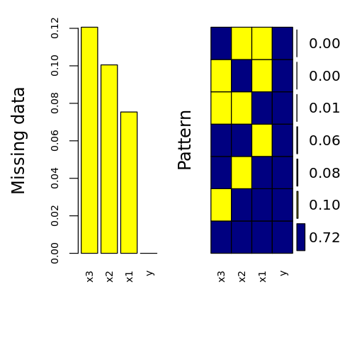
[20]:
p <- aggr(
    D.V,
    col=c('navyblue','yellow'),
    numbers=TRUE,
    sortVars=TRUE,
    labels=names(D.V),
    cex.axis=.7,
    gap=3,
    ylab=c('Missing data', 'Pattern')
)
 Variables sorted by number of missings:
 Variable      Count
       x3 0.12060302
       x2 0.10050251
       x1 0.07537688
        y 0.00000000
6.5. One-hot encoding
We perform one-hot encoding OHE on the categorical variables and store the result in D.O. Note how we start the training pipeline at OHE. The reason is to avoid data leakage. Had we applied OHE to the whole dataset, we might bias the training process toward better results.
[21]:
ohe <- dummyVars(~ ., data=D.T[,-4], sep='_')
D.O <- data.frame(predict(ohe, newdata=D[,-4]))
D.O$y <- D$y
[22]:
print(head(D.O))
          x1         x2 x3_blue x3_green x3_red   y
1  0.1247540  0.4817417       0        1      0 pos
2  0.3820746  0.8176848       0        1      0 pos
3  0.5792428 -0.3254274       1        0      0 pos
4 -0.2937481 -0.2674061       0        0      1 pos
5 -0.8283492  1.7163252       1        0      0 pos
6 -0.3327136  1.2376945       1        0      0 pos
[23]:
print(summary(D.O))
       x1                x2              x3_blue         x3_green
 Min.   :-2.8613   Min.   :-3.28763   Min.   :0.000   Min.   :0.000
 1st Qu.:-0.6961   1st Qu.:-0.59550   1st Qu.:0.000   1st Qu.:0.000
 Median :-0.0339   Median : 0.06348   Median :1.000   Median :0.000
 Mean   :-0.0184   Mean   : 0.03492   Mean   :0.502   Mean   :0.257
 3rd Qu.: 0.6836   3rd Qu.: 0.69935   3rd Qu.:1.000   3rd Qu.:1.000
 Max.   : 3.8147   Max.   : 3.17901   Max.   :1.000   Max.   :1.000
     x3_red        y
 Min.   :0.000   neg:394
 1st Qu.:0.000   pos:606
 Median :0.000
 Mean   :0.241
 3rd Qu.:0.000
 Max.   :1.000
6.6. Imputation
We will preprocess the training data using k-nearest neighbor imputation and store the result in D.I.
[24]:
library('RANN')

imp <- preProcess(D.O, method='knnImpute')
D.I <- predict(imp, newdata=D.O)

print(anyNA(D.I))
[1] FALSE
[25]:
print(head(D.I))
          x1         x2    x3_blue   x3_green    x3_red   y
1  0.1408176  0.4391669 -1.0035059  1.6994586 -0.563210 pos
2  0.3939391  0.7693556 -1.0035059  1.6994586 -0.563210 pos
3  0.5878898 -0.3541760  0.9955098 -0.5878343 -0.563210 pos
4 -0.2708553 -0.2971486 -1.0035059 -0.5878343  1.773761 pos
5 -0.7967326  1.6526029  0.9955098 -0.5878343 -0.563210 pos
6 -0.3091849  1.1821708  0.9955098 -0.5878343 -0.563210 pos
[26]:
print(summary(D.I))
       x1                 x2              x3_blue           x3_green
 Min.   :-2.79652   Min.   :-3.26564   Min.   :-1.0035   Min.   :-0.5878
 1st Qu.:-0.66661   1st Qu.:-0.61962   1st Qu.:-1.0035   1st Qu.:-0.5878
 Median :-0.01525   Median : 0.02807   Median : 0.9955   Median :-0.5878
 Mean   : 0.00000   Mean   : 0.00000   Mean   : 0.0000   Mean   : 0.0000
 3rd Qu.: 0.69053   3rd Qu.: 0.65305   3rd Qu.: 0.9955   3rd Qu.: 1.6995
 Max.   : 3.77058   Max.   : 3.09023   Max.   : 0.9955   Max.   : 1.6995
     x3_red          y
 Min.   :-0.5632   neg:394
 1st Qu.:-0.5632   pos:606
 Median :-0.5632
 Mean   : 0.0000
 3rd Qu.:-0.5632
 Max.   : 1.7738
6.7. Rescale
Let’s rescale the variables into the range [0, 1] and store the result in D.R.
[27]:
ran <- preProcess(D.I, method='range')
D.R <- predict(ran, newdata=D.I)
[28]:
print(head(D.R))
         x1        x2 x3_blue x3_green x3_red   y
1 0.4472809 0.5828955       0        1      0 pos
2 0.4858248 0.6348457       0        1      0 pos
3 0.5153584 0.4580750       1        0      0 pos
4 0.3845938 0.4670474       0        0      1 pos
5 0.3045163 0.7738113       1        0      0 pos
6 0.3787572 0.6997959       1        0      0 pos
[29]:
print(summary(D.R))
       x1               x2            x3_blue         x3_green
 Min.   :0.0000   Min.   :0.0000   Min.   :0.000   Min.   :0.000
 1st Qu.:0.3243   1st Qu.:0.4163   1st Qu.:0.000   1st Qu.:0.000
 Median :0.4235   Median :0.5182   Median :1.000   Median :0.000
 Mean   :0.4258   Mean   :0.5138   Mean   :0.502   Mean   :0.257
 3rd Qu.:0.5310   3rd Qu.:0.6165   3rd Qu.:1.000   3rd Qu.:1.000
 Max.   :1.0000   Max.   :1.0000   Max.   :1.000   Max.   :1.000
     x3_red        y
 Min.   :0.000   neg:394
 1st Qu.:0.000   pos:606
 Median :0.000
 Mean   :0.241
 3rd Qu.:0.000
 Max.   :1.000
[30]:
print(dim(D.R))
[1] 1000 6
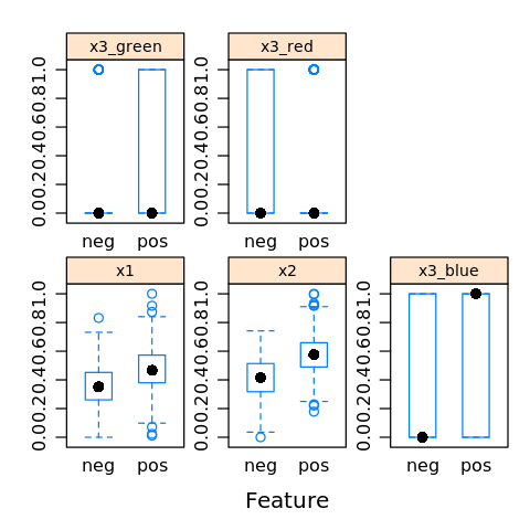
6.8. Feature importance
We may visualize feature importance to see which features/variables are important to the class variable.
[31]:
featurePlot(x=D.R[,1:5],
            y=D.R$y,
            plot='box',
            strip=strip.custom(par.strip.text=list(cex=.7)),
            scales = list(x = list(relation='free'),
                          y = list(relation='free')))
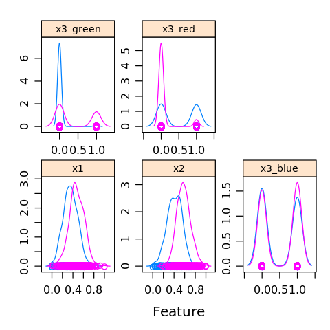
[32]:
featurePlot(x=D.R[,1:5],
            y=D.R$y,
            plot='density',
            strip=strip.custom(par.strip.text=list(cex=.7)),
            scales = list(x = list(relation='free'),
                          y = list(relation='free')))
6.9. Feature selection
Feature selection may help us to use only features (variables) that are important to the classification.
[33]:
ctrl <- rfeControl(
    functions=rfFuncs,
    method='repeatedcv',
    repeats=5,
    verbose=FALSE
)

profile <- rfe(y ~ ., data=D.R, sizes=c(2, 3), rfeControl=ctrl)
[34]:
profile
Recursive feature selection

Outer resampling method: Cross-Validated (10 fold, repeated 5 times)

Resampling performance over subset size:

 Variables Accuracy  Kappa AccuracySD KappaSD Selected
         2   0.8028 0.5861    0.03459 0.07315
         3   0.8102 0.5908    0.03654 0.08220
         5   0.8214 0.6186    0.03640 0.08056        *

The top 5 variables (out of 5):
   x2, x1, x3_red, x3_green, x3_blue
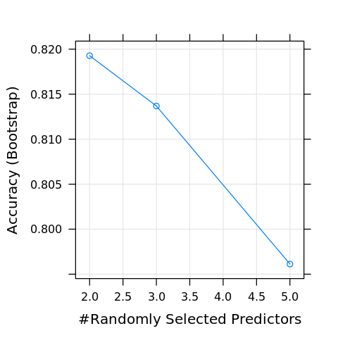
6.10. Training
We are now ready to train a classification model. We will use a random forest to classify the data. Use the modelLookup function to see which arguments are available. Below, the mtry argument/parameter is available. The model will be bound to M.
[35]:
modelLookup('rf')
| model | parameter | label | forReg | forClass | probModel |
|---|---|---|---|---|---|
| <chr> | <fct> | <fct> | <lgl> | <lgl> | <lgl> |
| rf | mtry | #Randomly Selected Predictors | TRUE | TRUE | TRUE |
[36]:
M <- train(y ~ ., data=D.R, method='rf')
[37]:
print(M)
Random Forest

1000 samples
   5 predictor
   2 classes: 'neg', 'pos'

No pre-processing
Resampling: Bootstrapped (25 reps)
Summary of sample sizes: 1000, 1000, 1000, 1000, 1000, 1000, ...
Resampling results across tuning parameters:

  mtry  Accuracy   Kappa
  2     0.8192793  0.6111993
  3     0.8136866  0.6049471
  5     0.7961271  0.5705189

Accuracy was used to select the optimal model using the largest value.
The final value used for the model was mtry = 2.
We may visualize the accuracy of the training with the predictors varying.
[38]:
plot(M)
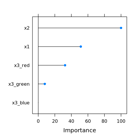
We may visualize the variable importance.
[39]:
vi <- varImp(M)
plot(vi)
6.11. Predicting on validation data
6.11.1. Transform validation data
We will not run the validation data D.V through the pipeline.
one-hot encoding,
Oimputation,
Iscaling (to the range [0, 1]),
R
[40]:
O <- predict(ohe, newdata=D.V)
[41]:
I <- predict(imp, newdata=O)
[42]:
R <- predict(ran, newdata=I)
[43]:
print(head(R))
          x1        x2 x3_blue x3_green x3_red
4  0.3845938 0.4670474       0        0      1
6  0.3787572 0.6997959       1        0      0
26 0.3598337 0.7515544       1        0      0
29 0.1134421 0.6750376       1        0      0
33 0.5267653 0.4183815       1        0      0
36 0.4480240 0.5460396       0        1      0
[44]:
print(dim(R))
[1] 199 5
6.11.2. Confusion matrix
Let’s look at the confusion matrix.
[45]:
y <- predict(M, R)
cm <- confusionMatrix(reference=D.V$y, data=y, positive='pos')
[46]:
print(cm)
Confusion Matrix and Statistics

          Reference
Prediction neg pos
       neg  62  16
       pos  16 105

               Accuracy : 0.8392
                 95% CI : (0.7806, 0.8873)
    No Information Rate : 0.608
    P-Value [Acc > NIR] : 1.118e-12

                  Kappa : 0.6626

 Mcnemar's Test P-Value : 1

            Sensitivity : 0.8678
            Specificity : 0.7949
         Pos Pred Value : 0.8678
         Neg Pred Value : 0.7949
             Prevalence : 0.6080
         Detection Rate : 0.5276
   Detection Prevalence : 0.6080
      Balanced Accuracy : 0.8313

       'Positive' Class : pos
6.11.3. Receiver operating characteristic curve
Let’s look at the area under the curve (AUC) for the Receiver Operating Characteristic curve.
[47]:
library('PRROC')

y <- predict(M, R, type='prob')[,1]

results <- data.frame(
    y = D.V$y,
    y.pred = y
)

class.0 <- results %>% filter(y == 'neg') %>% select(y.pred)
class.1 <- results %>% filter(y == 'pos') %>% select(y.pred)
[48]:
roc <- roc.curve(
    scores.class0=class.0$y.pred,
    scores.class1=class.1$y.pred,
    curve=TRUE,
    rand.compute=TRUE)

plot(roc, legend=1, rand.plot=TRUE)

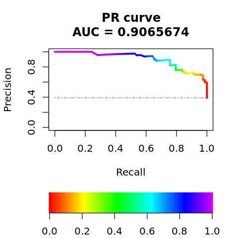
6.11.4. Precision-recall curve
The precision-recall curve is shown below.
[49]:
pr <- pr.curve(
    scores.class0=class.0$y.pred,
    scores.class1=class.1$y.pred,
    curve=TRUE,
    rand.compute=TRUE)

plot(pr, legend=1, rand.plot=TRUE)