3. Data Distributions

set.seed(37)

3.1. Normal distribution

The following are functions dealing with the normal distribution.

• rnorm samples from the normal distribution

• pnorm returns the probability of a sample (quantile)

• qnorm returns the quantile for a given probability

• dnorm returns the density function for an array of values

The rnorm function simply samples data points.

s <- rnorm(10, mean=0, sd=1)
print(s)

 [1]  0.1247540  0.3820746  0.5792428 -0.2937481 -0.8283492 -0.3327136
 [7] -0.1921595  1.3629827  0.8559544  0.2159955

The pnorm function gives you the cummulative probability up to the specified quantile.

p <- pnorm(c(-1.0, -0.4, -0.3, -0.2, -0.1, 0.0, 0.1, 0.2, 0.3, 0.4, 1.0), mean=0, sd=1)
print(p)

 [1] 0.1586553 0.3445783 0.3820886 0.4207403 0.4601722 0.5000000 0.5398278
 [8] 0.5792597 0.6179114 0.6554217 0.8413447

The qnorm function maps the quantile probability back to the quantile.

q <- qnorm(p, mean=0, sd=1)
print(q)

 [1] -1.0 -0.4 -0.3 -0.2 -0.1  0.0  0.1  0.2  0.3  0.4  1.0

The dnorm function gives the probability of the data point.

d <- dnorm(s, mean=0, sd=1)
print(d)

 [1] 0.3958498 0.3708606 0.3373280 0.3820963 0.2830817 0.3774611 0.3916443
 [8] 0.1575835 0.2765766 0.3897438

3.2. Other distributions

There are other distributions besides the normal distribution. They have the corresponding functions as with the normal distribution.

• r

• p

• q

• d

command	distribution
dbeta	beta
dbinom	binomial
dcauchy	Cauchy
dchisq	chi-squared
dexp	exponential
df	F distribution
dgamma	gamma
dgeom	geometric
dhyper	hypergeometric
dlnorm	log-normal
dmultinom	multinomial
dnbinom	negative binomial
dnorm	normal
dpois	Poisson
dt	Student’s t
dunif	uniform distribution
dweibull	Weibull
dwilcox	Wilcoxon rank sum
ptukey	Studentized range
dsignrank	Wilcoxon signed rank

3.3. Normality test

You may use the Shapiro-Wilk Test to test for normality. Below, we sample from a normal distribution and test for normality. Note that the p-value is greater than (let’s say) 0.05, and so we fail to reject the null hypothesis (there is no difference between the normal distribution and the one observed).

x <- rnorm(1000, m=0, sd=1)
r <- shapiro.test(x)
print(r)

        Shapiro-Wilk normality test

data:  x
W = 0.99869, p-value = 0.6793

Now, we sample from a Poisson distribution and apply the normality test. The p-value is less than 0.05 and so we reject the null hypothesis in favor the the alternative one (there is a difference between the normal distribution and the one observed).

x <- rpois(1000, lambda=3)
r <- shapiro.test(x)
print(r)

        Shapiro-Wilk normality test

data:  x
W = 0.94566, p-value < 2.2e-16

3.4. Comparing two distributions

We may use the Kolmogorov-Smirnov Test (or KS Test) to test if two distributions are the same.

x <- rnorm(1000, m=0, sd=1)
y <- rnorm(1000, m=0, sd=1)
r <- ks.test(x, y)
print(r)

        Two-sample Kolmogorov-Smirnov test

data:  x and y
D = 0.032, p-value = 0.6852
alternative hypothesis: two-sided

The KS Test may also be called with a probability function. Below, we use pnorm to test if the distribution of x follows a normal distribution with mean 0 and standard deviation 1.

x <- rnorm(1000, m=0, sd=1)
r <- ks.test(x, 'pnorm', mean=0, sd=1)
print(r)

        One-sample Kolmogorov-Smirnov test

data:  x
D = 0.02782, p-value = 0.4213
alternative hypothesis: two-sided

Now we compare with a normal distribution with mean 5 and standard deviation 1.

x <- rnorm(1000, m=5, sd=1)
r <- ks.test(x, 'pnorm', mean=0, sd=1)
print(r)

        One-sample Kolmogorov-Smirnov test

data:  x
D = 0.98743, p-value < 2.2e-16
alternative hypothesis: two-sided

Here, we use ppois to test if the distribution of x follows a Poisson distribution with lambda 5.

x <- rnorm(1000, m=0, sd=1)
r <- ks.test(x, 'ppois', 5)
print(r)

        One-sample Kolmogorov-Smirnov test

data:  x
D = 0.93457, p-value < 2.2e-16
alternative hypothesis: two-sided

3.5. Quantile-Quantile Plot

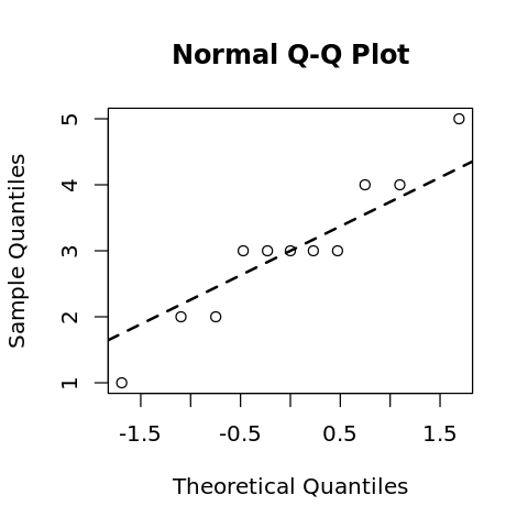
The Quantile-Quantile Plot (QQ Plot) is a visual way to also test for normality. To idea is to see if the data points fall on the straight line.

3.5.1. qqnorm

The qqnorm function provides a way to visually tests if a distribution is normal. Note the use of qqline to draw the straight line.

x <- c(1, 2, 2, 3, 3, 3, 3, 3, 4, 4, 5)

options(repr.plot.width=4, repr.plot.height=4)

qqnorm(x)
qqline(x, lwd=2, lty=2)

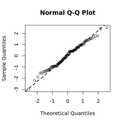
Here, we sample from a normal distribution and form a QQ Plot. Note that the data falls nearly on the straight line.

x <- rnorm(100, m=0, sd=1)

options(repr.plot.width=4, repr.plot.height=4)

qqnorm(x)
qqline(x, lwd=2, lty=2)

3.5.2. qqplot

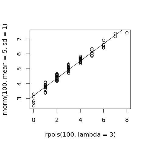
The qqplot function may be used to compare two distributions. Below, we compare the distribution of data coming from a Poisson distribution to that coming from a normal distribution.

options(repr.plot.width=4, repr.plot.height=4)

p <- qqplot(rpois(100, lambda=3), rnorm(100, mean=5, sd=1))
abline(lm(p$y ~ p$x))

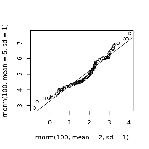
Here, we compare two normal distributions parameterized differently.

options(repr.plot.width=4, repr.plot.height=4)

p <- qqplot(rnorm(100, mean=2, sd=1), rnorm(100, mean=5, sd=1))
abline(lm(p$y ~ p$x))

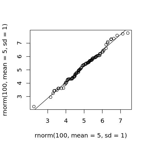
Here, we compare two normal distributions parameterized the same.

options(repr.plot.width=4, repr.plot.height=4)

p <- qqplot(rnorm(100, mean=5, sd=1), rnorm(100, mean=5, sd=1))
abline(lm(p$y ~ p$x))